MDS in Action

Recent Developments and Implementation

Patrick Mair, Harvard University

2023-12-06

Menu

In this talk I focus on some recent developments in multidimensional scaling and unfolding:

• Multidimensional scaling (MDS):
  • Quick intro and theory: example, purpose, data structures, stress, interpretation.
  • Goodness-of-fit assessment: some diagnostics and tools.
  • Interpretation: facet-based interpretation using support vector machines, biplots.
  • Procrustes and some MDS variants.
• Unfolding:
  • Quick intro and theory: example, purpose, data structures, stress, interpretation.
  • Row-conditional unfolding and other unfolding variants.

All these methods and developments are implemented in the smacof package.

De Leeuw, J., & Mair, P. (2009). Multidimensional Scaling Using Majorization: SMACOF in R. Journal of Statistical Software, 31(3), 1-30. DOI: 10.18637/jss.v031.i03

Mair, P., Groenen, P. J. F., and De Leeuw, J. (2022). More on multidimensional scaling in R: smacof version 2. Journal of Statistical Software, 102(10), 1-47. DOI: 10.18637/jss.v102.i10

Multidimensional Scaling

Example

Dataset taken from McNally et al. (2017) involving PTSD symptoms reported by survivors of the 2008 Wenchuan earthquake in China using the PTSD checklist-civilian version (PCL-C), included in the MPsychoR package. All 17 items were scaled on a 5-point Likert scale (1 … not at all; 5 … extremely). We have a sample size 362 persons.

intrusion	dreams	flash	upset	physior	avoidth	avoidact	amnesia	lossint	distant	numb	future	sleep	anger	concen	hyper	startle
2	2	2	2	3	2	3	2	3	2	2	1	3	4	3	4	2
2	2	2	3	3	3	3	2	3	3	2	2	3	3	2	3	3
2	4	4	4	3	3	3	5	4	3	2	3	4	4	4	3	4
2	1	2	2	1	1	2	2	2	1	1	2	2	1	2	3	3
2	2	2	2	2	2	2	2	3	2	2	2	3	2	3	2	3
4	3	2	2	2	2	3	3	2	2	2	3	2	3	2	3	2

Example

We start with computing a correlation matrix, subsequently converted into a dissimilarity matrix and fed into smacof’s mds() function, fitting a 2D solution:

delta <- cor(Wenchuan, use = "pairwise.complete.obs") |> sim2diss()
fit_mds <- mds(delta, type = "ordinal")

print(fit_mds)

Call:
mds(delta = delta, type = "ordinal")

Model: Symmetric SMACOF 
Number of objects: 17 
Stress-1 value: 0.145 
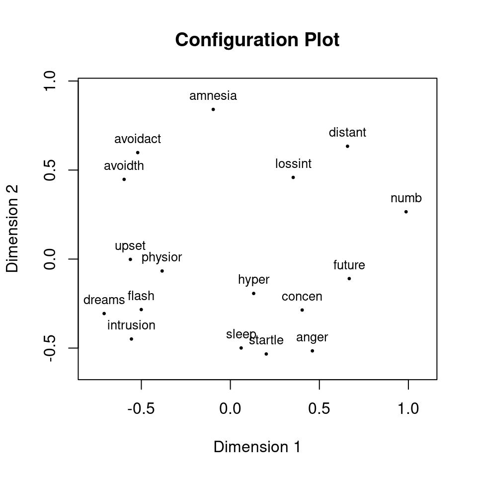
Number of iterations: 22 

We get a normalized stress value of 0.145 indicating how well the solution fits. Then we plot the configuration showing how the PTSD symptoms are related to each other (i.e., we create a map of the objects).

plot(fit_mds)

Input Structure

If we need a definition: “MDS is a technique that represents proximities among objects as distances among points in a low-dimensional space (with given dimensionality).” It allows researchers to explore similarity structures among objects in a multivariate dataset.

Standard textbook:
Borg I., & Groenen, P. J. F. (2005). Modern Multidimensional Scaling: Theory and Applications (2nd ed). New York: Springer.

Let us now focus on the building blocks of an MDS fit, and start with the input data:

• Derived dissimilarities based on multivariate dataset: popular options are dissimilarities derived from a correlation matrix, direct computation of Euclidean distance matrix using dist(), or any other dissimilarity measure that is suits the nature of the input data (see proxy package).
• Observed dissimilarities: experimental setup where participants judge how (dis)similar stimuli are (e.g., perceived color similarities in psychophysics).

In either case we organize the data in an \(n \times n\) matrix \(\Delta\) (\(n\) as the number of objects) with elements \(\delta_{ij}\).

Theory

The most popular MDS loss function to be minimized is the stress:

\[\sigma(\hat{\mathbf D},\mathbf X) = \sum_{i < j} w_{ij}(\hat{d}_{ij} - d_{ij}(\mathbf X))^2 \rightarrow \text{min!}\]

with the constraint \(\sum_{i < j} w_{ij}\hat{d}_{ij}^2 = n(n-1)/2\), further normalized to stress-1.

• \(\mathbf X\) as the \(n \times p\) configuration matrix containing the point coordinates in the \(p\)-dimensional space (\(p\) is usally 2 or 3), with \(d_{ij}(\mathbf X) = \sqrt{\sum_{s=1}^p (x_{is} - x_{js})^2}\) as the fitted Euclidean distances.
• \(w_{ij}\) are some optional a priori weights (e.g., for blanking out missings during optimization).
• The \(\hat d_{ij}\)’s (with corresponding \(n \times n\) matrix \(\hat{\mathbf D}\)) are called disparities or d-hats, based on an optimal scaling transformation¹.
  • Ratio MDS: \(\hat{d}_{ij} = b\delta_{ij}\).
  • Interval MDS: \(\hat{d}_{ij} = a + b\delta_{ij}\).
  • Monotone spline MDS: \(\hat{d}_{ij} = f(\delta_{ij})\) where \(f\) is an \(I\)-spline (integrated spline) transformation with fixed number of knots and spline degree.
  • Ordinal MDS: \(\hat{d}_{ij} = f(\delta_{ij})\) where \(f\) is a monotone step function with options for primary or secondary handling of ties.

Optimization

In SMACOF, stress is minimized using majorization:

• We use a Torgerson scaling¹ as starting solution a starting solution (cmdscale() in R).
• Using a quadratic surrogate function, majorization aims to find the minimum of the stress surface.
• Problem: The stress surface is bumpy and the algorithm may end up in a local minimum.

Borg and Mair (2017) proposed a simple multi-step approach involving multiple random starts and Procrustean alignment, emphasizing the interpretability of the resulting configuration.

Remark:
The lower the number of dimension \(p\), the more serious the local minimum problem. For the extreme case of \(p=1\) (unidimensional scaling, see Mair & De Leeuw, 2015) we’ve implemented the uniscale() function which runs through all the \(n!\) dissimilarity permutations a returns the solution with the lowest stress (works for a small \(n\) only, obviously).

Stability of a Solution

For derived dissimilarity setups, one can use a jackknife or a bootstrap to assess the stability of a solution, leading to confidence ellipses around the points in the configuration.

set.seed(123)
boot_wen <- bootmds(fit_mds, data = Wenchuan, 
                    method.dat = "pearson", nrep = 500)
boot_wen

Call: bootmds.smacofB(object = fit_mds, data = Wenchuan, method.dat = "pearson", 
    nrep = 500)

SMACOF Bootstrap:
Number of objects: 17 
Number of replications: 500 

Mean bootstrap stress:  0.1607 
Stress percentile CI:
  2.5%  97.5% 
0.1291 0.1982 

Stability coefficient: 0.9047 

Other parametric approaches:

• Pseudo confidence ellipses based on second stress derivations (de Leeuw, 2019);
• Log-normal framework with ML estimation (Ramsay, 1982), see smacofx package.
• Bayesian MDS (Oh & Raftery, 2001), see bayMDS package.

plot(boot_wen)

Goodness-of-Fit Assessment

People often simply apply Kruskal’s stress rules of thumb (0.20 “poor”, 0.1 “fair”, 0.05 “good”, 0.025 “excellent”, 0 “perfect”). Aside from the fact that these rules are problematic for various reasons (e.g., \(n\) as well as number of missings influence the stress magnitude), goodness-of-fit assessment in MDS is more multi-faceted (Mair, Borg, and Rusch, 2016):

• Dimensionality \(p\): Usually kept at \(p = 2\) or \(3\), but if one is willing to sacrifice a the option to plot 2D or 3D, a scree plot with (\(p\) on the x-axis, stress on the y-axis) can be used.
• Choice of transformation function \(\hat d_{ij}\): An ordinal solution always fits better than an interval or ratio, but might overfit or lead to a degenerate configuration. Shepard plots can be used to visually assess and judge the choice of transformation.
• Influential points: For each point we can determine its contribution to the stress value (stress-per-point SPP). Points that contribute highly can be eliminated.
• Interpretability of a solution.

Goodness-of-Fit Assessment

Various transformation functions applied to the Wenchuan data. Shepard plots:

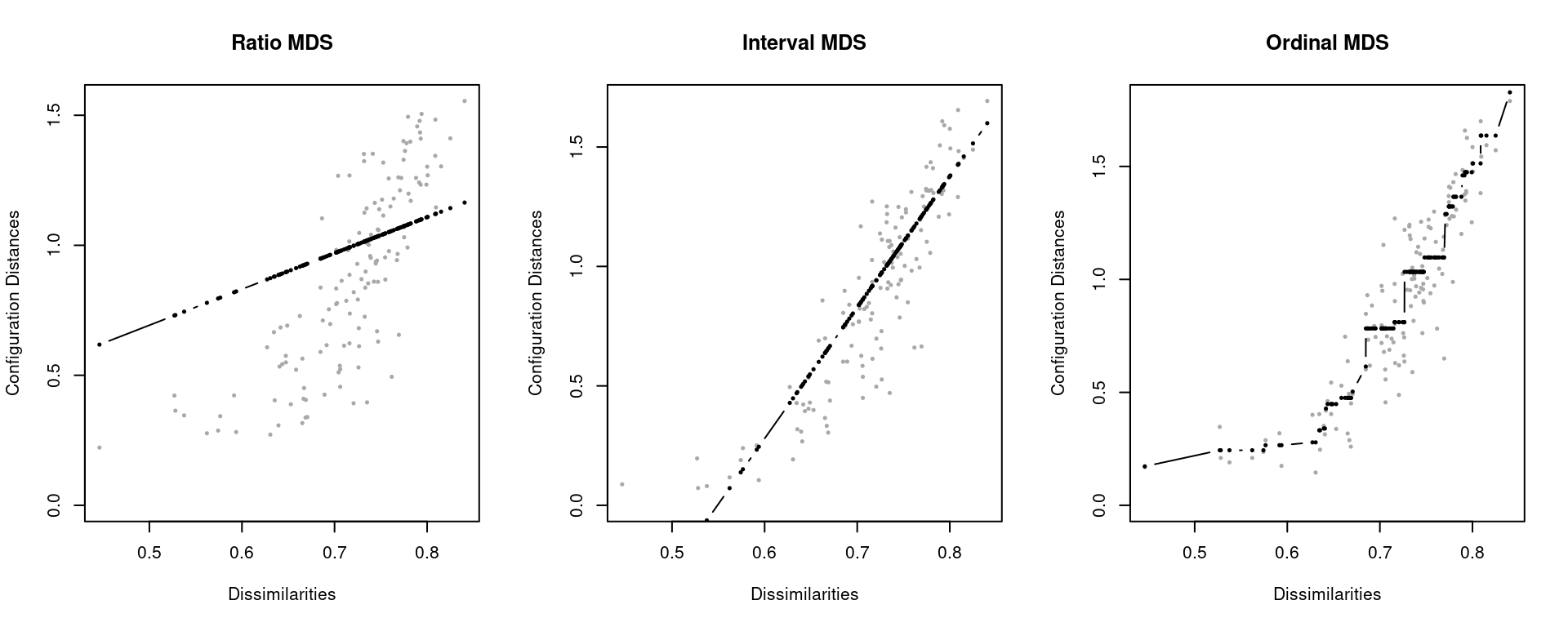
The choice of the transformation function can be made in a data-driven way (Shepard plots), or ad hoc depending on the nature of the input data.
It holds that ordinal stress \(\leq\) interval stress \(\leq\) ratio stress.

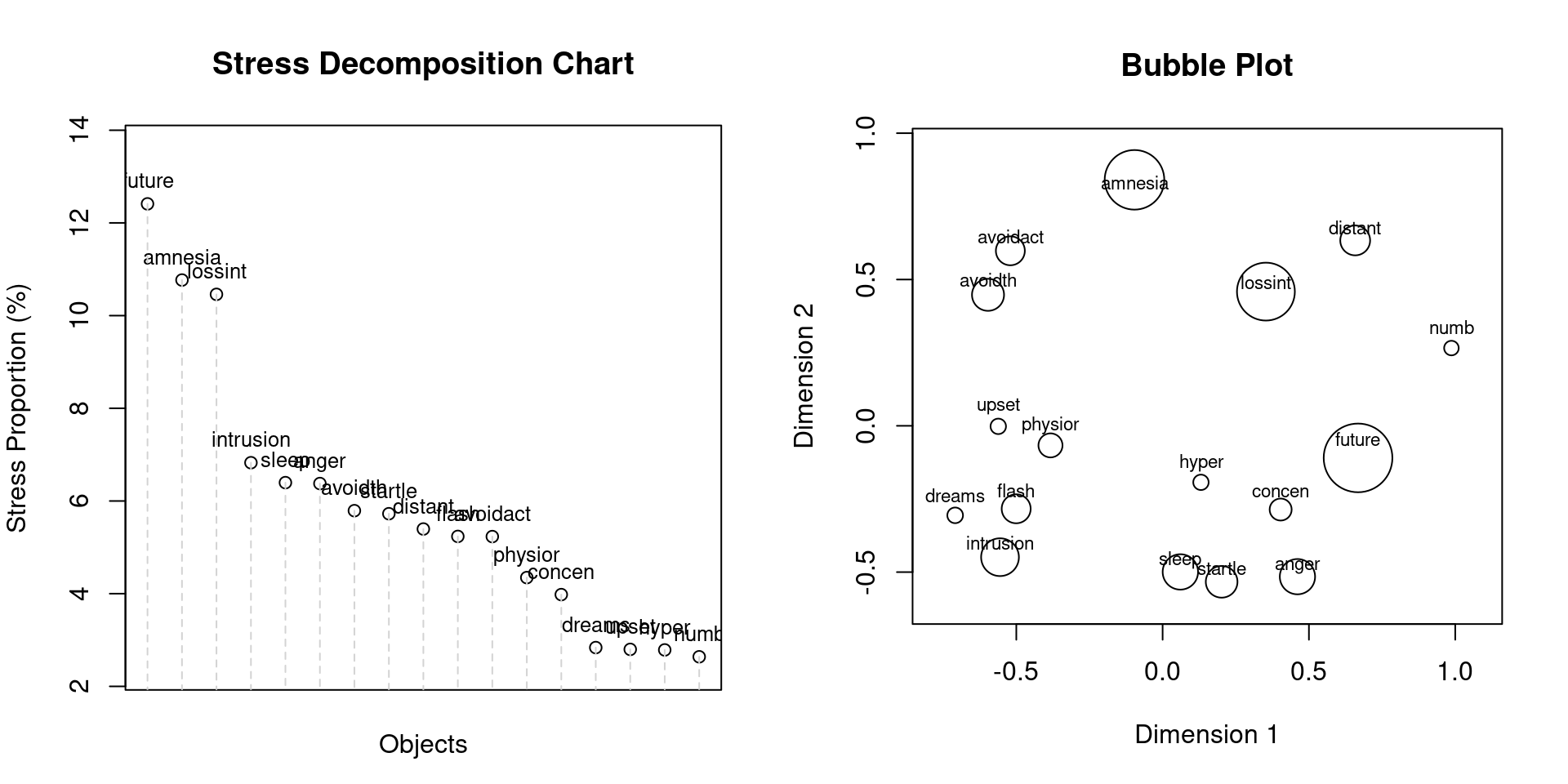
Goodness-of-Fit Assessment

SPP plots: SPP decomposition in percentages, and incorporating the SPP information into the configuration plot (the larger the circle, the larger the SPP):

Interpretation I

As opposed to PCA, there’s usually less focus on interpreting the dimensions in the configuration plot since the solution can be rotated arbitrarily¹.

Interpretation options:

• Distances between objects in the configuration plot (most common interpretation).
• Clustering points in the configuration (e.g., a hierarchical cluster analysis on the fitted distance matrix).
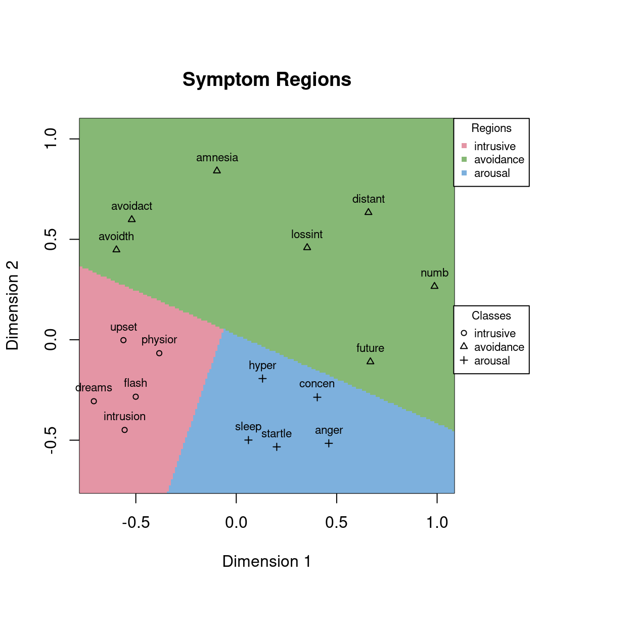
• Partitioning the MDS space using SVM in case we have labels for the objects². The plot to the right shows a linear SVM-based facet partitioning using the DSM-IV labels.

Interpretation II

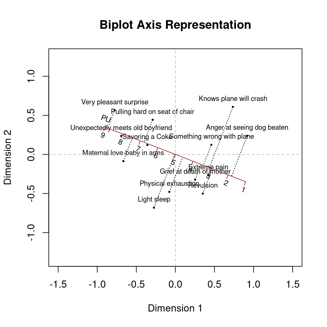
Having object covariates, we can map corresponding axes onto the configuration (either as vector or as actual axes with projections for which the calibrate package comes in handy). This is called an MDS biplot^1,2.

MDS biplots solve the multivariate regression problem

\[\mathbf Y = \mathbf{XB} + \mathbf E\]

with \(\mathbf Y\) as an \(n \times q\) of external covariates, and \(\mathbf X\) the MDS configuration. The resulting \(\hat{\mathbf B}\) determines the new axes.

Example:

• Participants had to rate proximities of 13 facial expressions (directly observed proximities).
• Rating scale values were collected for a “pleasant-unpleasant” (PU) covariate.

Procrustes

Let us assume we have two MDS configurations with the same objects but coming from two different conditions. The two resulting configurations may be aligned quite differently due to the “arbitrariness” of the dimensional alignment. This is where Procrustes¹ (“the stretcher who hammers out the metal”) comes in.

The goal of Procrustes is to align a testee configuration with a target configuration by removing “meaningless” differences (i.e., translation, rotation, and dilation which don’t change the stress value of a solution).

Procrustes Example

We have two dissimilarity matrices of work values from former West and East Germany. We start with fitting two separate MDS solutions, subsequently aligned with Procrustes (with East Germany as target configuration).

fit_east <- mds(eastD, type = "ordinal")
fit_west <- mds(westD, type = "ordinal")
fit_proc <- Procrustes(X = fit_east$conf, Y = fit_west$conf)
fit_proc

Call: Procrustes(X = fit_east$conf, Y = fit_west$conf)

Congruence coefficient: 0.951
Alienation coefficient: 0.308
Correlation coefficient: 0.666

Rotation matrix:
       D1     D2
D1 -0.990 -0.139
D2  0.139 -0.990

Translation vector: 0 0 
Dilation factor: 0.672 

round(fit_proc$pairdist, 3)[1:10]

               Work useful for society   Work that is meaningful and sensible 
                                 0.005                                  0.072 
                      Interesting work           Good chances for advancement 
                                 0.199                                  0.250 
Work that requires much responsibility         Work where one can help others 
                                 0.260                                  0.265 
                      Independent work  Work that is recognized and respected 
                                 0.273                                  0.332 
                           High income             Healthy working conditions 
                                 0.354                                  0.372 

MDS Variants

Constrained MDS and 3-way MDS approaches (both implemented in smacof):

• External constraints: confirmatory MDS with optimal scaling on external covariates.
• Internal constraints: spherical constraints on the configuration (e.g., points are arranged on a circle in 2D).
• INDSCAL and IDIOSCAL: list of dissimilarity matrices as input.

Structure optimized scaling:

• Cluster optimized proximity scaling (cops package; Rusch et al., 2021): incorporating clusteredness into an MDS configuration.
  
• Structure optimized proximity scaling (stops package; Rusch et al., 2023): extending COPS to other structures.

Other MDS approaches like Multiscale, ALSCAL, Box-Cox MDS, local MDS, POST-MDS etc. are implemented in the smacofx package.

Conceptually related methods are t-SNE (nonlinear, local structure preserving) and UMAP (nonlinear, local and global structure preserving), popular in NLP for dimensionality reduction and visualization of word embeddings.

Unfolding

Example

Unfolding takes one the following two data structures:

(Partial) rankings:

head(carconf1)

  price exterior brand tech.equip country interior
1     3        2     5          6       4        1
2     4        1     5          2       6        3
3     6        3     2          5       4        1
4     1        4     2          3       6        5
5    NA        2     4         NA       3        1
6    NA        2     4          3      NA        1

Ratings:

head(lik_dat)

  Item1 Item2 Item3 Item4 Item5
1     3     4     3     3     1
2     3     1     1     2     3
3     2     2     4     2     5
4     2     3     1     1     4
5     3     5     1     3     2
6     5     3     5     4     5

Note that in either case the values need to represent dissimilarities. E.g., having ratings and a value of 5 means “fully agree”, the scores needs to be reversed.

Here we proceed with the partial ranking example where 100 participants were asked to configure a car according to their preferences (taken from the prefmod package).

Example

Let us fit an ordinal unfolding solution on the car preference data:

fit_unf <- unfolding(carconf1, type = "ordinal") 
fit_unf

Call: unfolding(delta = carconf1, type = "ordinal")

Model:               Rectangular smacof 
Number of subjects:  100 
Number of objects:   6 
Transformation:      ordinalp 
Conditionality:      matrix 

Stress-1 value:    0.297371 
Penalized Stress:  2.330348 
Number of iterations: 135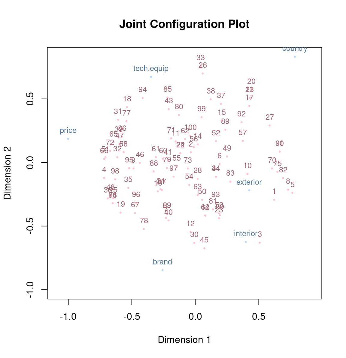 

plot(fit_unf)

Unfolding Theory

Historically, unfolding was treated separately from MDS (Coombs, 1964). With the development of the SMACOF theory in the 70s and 80s, unfolding can nowadays be seen as a variant of MDS taking a rectangular dissimilarity matrix as input.
The starting point is the following stress formulation for input matrix \(\boldsymbol{\Delta}\) of dimension \(n \times m\) with elements \(\delta_{ij}\) (\(i = 1,\ldots,n\) and \(j=1,\ldots,m\)):

\[\sigma^2(\hat{\mathbf D}, \mathbf X_1, \mathbf X_2) = \sum_{i=1}^n \sum_{j=1}^m w_{ij}(\hat d_{ij} - d_{ij}(\mathbf X_1, \mathbf X_2))^2\]

with the fitted Euclidean distances (\(p\)-dimensional space) expressed as \(d_{ij}(\mathbf X_1, \mathbf X_2) = \sqrt{\sum_{s=1}^p (x_{1is} - x_{2js})^2}\). \(\mathbf X_1\) is an \(n \times p\) matrix (row configuration), \(\mathbf X_2\) an \(m \times p\) matrix (column configuration), and \(\hat{\mathbf D}\) the \(n \times m\) matrix of disparities.

One major problem when incorporating transformations (e.g., ordinal in \(\hat d_{ij}\)) is degeneracy of the solution due to equal disparities. Busing et al. (2005) suggest to penalize the stress function by the coefficient of variation, which moves the algorithm away from solutions with small variation in the fitted distances.

Variants

The smacof package implements the following unfolding variants:

• Vector model of unfolding (Tucker, 1960): old geometric approach using an SVD on the input similarity matrix.
• External unfolding: use fixed, theory-driven coordinates for the rows or columns.
• Spherical unfolding: restrict either row coordinates or column coordinates to be on a geometric shape such as a sphere.
• Row-conditional unfolding: estimating a separate transformation function for each row (see below).

Remark: Goodness-of-fit in unfolding can be assessed in a similar way as in MDS (Mair et al., 2016).

Row-Conditional Unfolding

Unfolding, as introduced so far assumes a single transformation function across rows (individuals in our example). In certain situations, this can be fairly restrictive:

• Rankings: It might be the case that individual \(i\) is quite indifferent to all car characteristics, but still ranks them. Individual \(i'\), however, could have strong preferences but might end up with the same ranking as individual \(i\).
• Ratings: Some individuals may use the rating scale on which they express their preferences completely differently, e.g., by avoiding extreme ratings.

To account for such potential individual differences we are now going to fit an ordinal, row-conditional unfolding solution on the car preference data:

fit_unf2 <- unfolding(carconf1, type = "ordinal", conditionality = "row")

Row-Conditional Unfolding

The Shepard plot shows nicely the difference between an unconditional and a row-conditional solution:

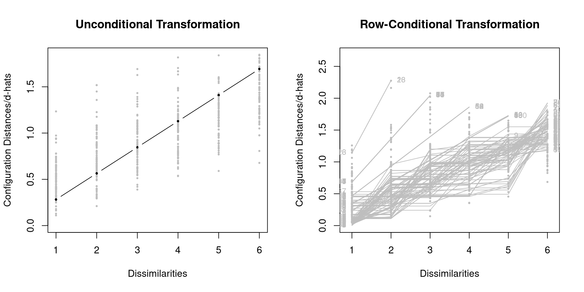
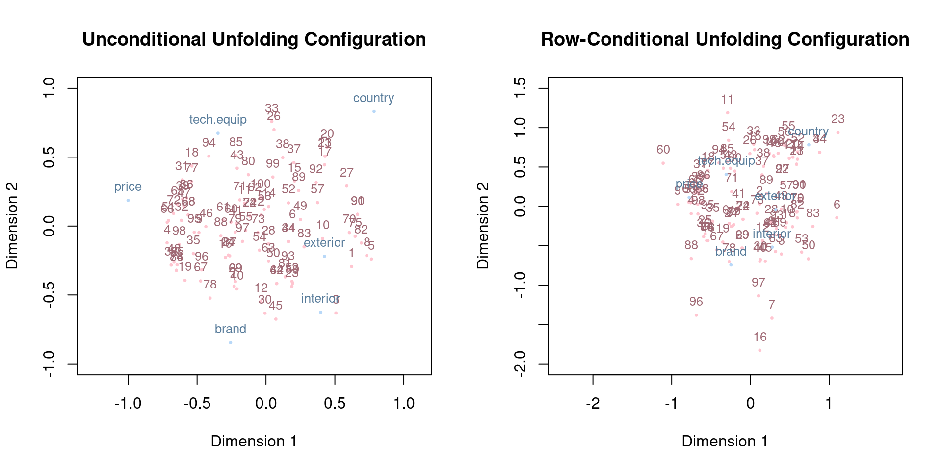
Row-Conditional Unfolding

We get a stress-1 value of 0.297 for the unconditional solution, and 0.203 for the row-conditional one. Let’s look at the configurations:

Summary

Takeaways: MDS is a widely applicable family of methods for scaling input dissimilarities, that is, we create a “map” of our data. We have focused on

• basic MDS on a symmetric input dissimilarity matrix (stability, goodness-of-fit assessment, interpretation of a solution) and Procrustes for aligning two or more configurations;
• unfolding on a rectangular input dissimilarity matrix (rankings, ratings) including row-conditionality.

Further details, applications, and related methods can be found in

Mair, P., Groenen, P. J. F., and De Leeuw, J. (2022). More on multidimensional scaling in R: smacof version 2. Journal of Statistical Software, 102(10), 1-47. DOI: 10.18637/jss.v102.i10

Mair, P. (2018). Modern Psychometrics with R. New York: Springer.